Function definitions
The bbob-mixint Suite
The bbob-mixint suite is constructed by partially discretizing problems from the bbob (Finck et al. 2009) and bbob-largescale (Varelas et al. 2018) suites. In the following, we first explain how the discretization is performed, then describe the construction of the suite and finally show how the functions are scaled to adjust their difficulty.
Discretization
Consider a bbob(or bbob-largescale) problem with the function f: \mathbb{R}^n \to \mathbb{R} and optimal value f^{\textrm{opt}} = f(\mathbf{x}^{\textrm{opt}}). The resulting mixed-integer function will have the form \overline{f}: \mathbb{Z}^k \times \mathbb{R}^{(n-k)} \to \mathbb{R}, that is, it will be defined on k integer and n-k continuous variables. While all bbob functions are defined for any \mathbf{x} \in \mathbb{R}^n, all but the linear slope function have their optimal solution within [-4, 4]^n. The partial discretization is performed in such a way that the optimal value is preserved, that is \vphantom{f}\smash{\overline f}^{\textrm{opt}} = f^{\textrm{opt}}.
Now let us assume that we wish to discretize the variable x_i, where i \in \{1, \dots, k\}, into the set \{0, \dots, l-1\} of l integer values. This discretization is done as follows:
First, we define a sequence of l equidistant auxiliary values -4 < y_1 < \cdots < y_l < 4 so that y_{j+1}-y_j=\frac{4+4}{l + 1}=y_1-(-4)=4-y_l, where j = 1, \dots, l - 1.
We denote with y^{*} the value y_j, j = 1, \dots, l, that is closest to x_i^{\text{opt}}. The difference between the two is represented by d_i = y^{*} - x_i^{\text{opt}}. Note that |d_i| \leq \frac{4}{l+1} if x_i^{\text{opt}} \in [-4, 4].
Then, z_j = y_j - d_i for j = 1, \dots, l. This aligns one of the z_j values with x_i^{\text{opt}}.
Finally, the following transformation \zeta is used to map any continuous value x_i \in \mathbb{R} to an integer in \{0, \dots, l-1\}: \zeta (x_i) = \left\{\begin{array}{cl} 0 &\quad\text{if}\quad x_i < z_1 + \frac{4}{l+1} \\[0.2em] 1 &\quad\text{if}\quad z_1 + \frac{4}{l+1} \leq x_i < z_2 + \frac{4}{l+1} \\ \vdots & \quad\vdots \\ l-1 &\quad\text{if}\quad z_{l-1} + \frac{4}{l+1} \leq x_i \end{array}\right.
The values y_j, j = 1, \dots, l, in Step (1) are chosen in such a way that the corresponding shifted values z_j remain within [-4, 4] if x_i^{\text{opt}} is also in [-4, 4]. If not, the shift is larger, but z_j, j = 1, \dots, l, never go beyond x_i^{\text{opt}}, which in practice means they remain within [-5, 5]^n—the region of interest for all bbob problems.
Suite Construction
The bbob suite consists of problems with 24 different functions in 6 dimensions, n = 2, 3, 5, 10, 20, 40, and 15 instances (see (Finck et al. 2009) for the function definitions). Because the discretization reduces the number of continuous variables, higher dimensions are used for the bbob-mixint suite to produce challenging problems. We chose n = 5, 10, 20, 40, 80, 160 as the dimensions of the bbob-mixint suite.1
Because the numerical effort for some bbob problems scales with n^2, we use these for dimensions \leq 40 only. For dimensions >40, we use the corresponding problems from the bbob-largescale suite (Varelas et al. 2018) which scale linearly with n.
As all dimensions n are multiples of 5, we define five arities for n/5 consecutive variables, respectively, as l=2,4,8,16,\infty. We use instances 1–15 to instantiate each problem. They match the equally-numbered instances of the underlying bbob and bbob-largescale problems.
Function Scaling
Initial experiments using the algorithms Random Search, CMA-ES (Hansen and Auger 2014) and DE (Storn and Price 1997) have shown that the new problems are of considerably different difficulties. Some are extremely hard to solve, while for others, a non-negligible percentage of targets is met already after a handful of function evaluations. Because COCO’s performance assessment aggregates results over function and target pairs, we scale function values to adjust for these different difficulties.
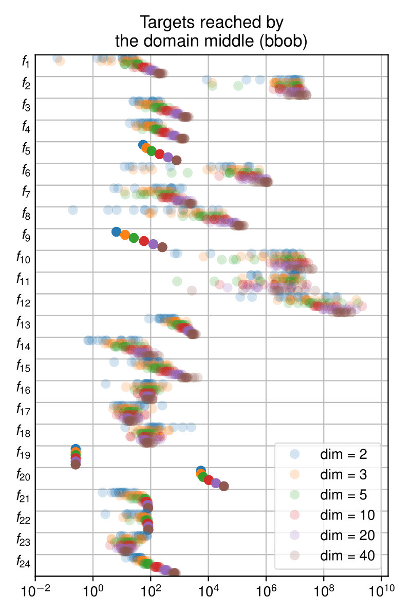
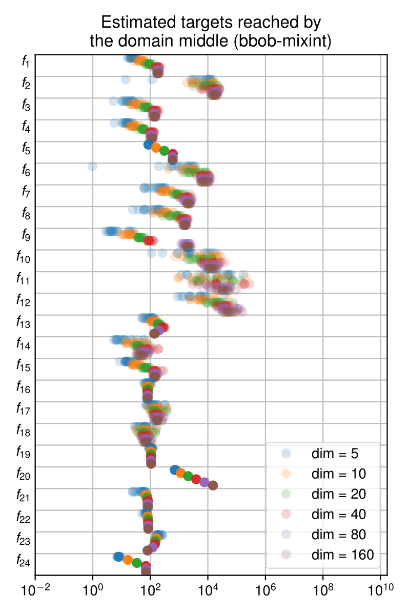
In order to decide on the scaling factors, we look at how many targets can be reached just by evaluating the domain middle (often the first guess of an optimization algorithm). However, because two values could be interpreted as the ‘middle’ value for variables of even arity, we need to sample among a large set of possible domain middle points. Figure 1 (b) shows the difference between the median f-value of 1000 domain middle samples and the f-value of the optimal solution for each problem instance in the bbob-mixint suite prior to scaling. In comparison, Figure 1 (a) shows the difference between the f-value of the domain middle and of the optimal solution for each problem instance for the bbob suite (note that no sampling is required here since it is clear which point is the domain middle in a continuous domain).
Keeping in mind that in COCO the easiest target defaults to 100, we see that for a number of bbob-mixint functions (f_2, f_6, f_{10} to f_{13} and f_{20}), the domain middle rarely (if ever) achieves this target. On the other hand, for functions such as f_{17}, f_{19} and f_{23}, evaluating the domain middle already guarantees reaching targets of 10 and less. We also see that the distances for the bbob-mixint suite are very similar to those for the bbob suite, albeit a bit larger in general. Based on these findings and the preliminary algorithm results, we choose to multiply the f-values of the functions with the scaling factors shown in Table. This setting is mindful of the connections between some functions, for example, the same scaling factors are used for the original (f_8) and rotated (f_9) Rosenbrock functions. Figure 1 (c) shows the result for all (scaled) bbob-mixint problems. Now the f-differences between the domain middle and the optimal solution are more uniform across the problems in the suite.

| Factor | Value | Factor | Value | Factor | Value | Factor | Value |
|---|---|---|---|---|---|---|---|
| f_1 | 1 | f_7 | 1 | f_{13} | 0.1 | f_{19} | 10 |
| f_2 | 10^{-3} | f_8 | 10^{-2} | f_{14} | 1 | f_{20} | 0.1 |
| f_3 | 0.1 | f_9 | 10^{-2} | f_{15} | 0.1 | f_{21} | 1 |
| f_4 | 0.1 | f_{10} | 10^{-3} | f_{16} | 1 | f_{22} | 1 |
| f_5 | 1 | f_{11} | 10^{-2} | f_{17} | 10 | f_{23} | 10 |
| f_6 | 10^{-2} | f_{12} | 10^{-4} | f_{18} | 1 | f_{24} | 0.1 |
To summarize, the bbob-mixint suite contains mixed-integer problems constructed by discretizing the continuous problems from the bbob and bbob-largescale suites. Using 24 functions, 6 dimensions and 15 instances results in the total of 2160 problem instances.
References
Footnotes
Note that the function definitions of all mentioned test suites are scalable in dimension. The six dimensions are only pre-chosen to facilitate the experimental setup.↩︎